Introduction

Strokes Gained is an interesting method for evaluating golfers, co-created by Columbia Business School professor Mark Broadie.

Strokes Gained co-creator @markbroadie illustrates the statistic using Justin Thomas' final-round eagle at the 2021 #THEPLAYERS. 🔎 pic.twitter.com/LJ6qnp3ooE
— Golf Channel (@GolfChannel) March 8, 2023

From my understanding, Strokes Gained is similar to Expected Points Added (EPA) in football - golfers are evaluated against an “expected” number of strokes remaining after each shot. This “expected” value is based off a predictive model trained on historical data¹. In this post, I’ll build an expected strokes remaining model using PGA ShotLink data, which can later be used to estimate strokes gained. The model will use features in the shot-level data to predict how many strokes remaining the golfer has before the shot.

Data Preparation

First, I’ll load the cleaned up data from my previous post.

library(tidyverse)
library(tidymodels)

shot_level <- readRDS("../02_shotlink_explore/shot_level.rds")
cut_colors <- readRDS("../02_shotlink_explore/cut_colors.rds")

Before I start building a model, I want to gain a better understanding of how penalties, drops, and provisionals are handled in the data. The shot_type_s_p_d column has this information (S = Shot, P = Penalty, D = Drop, Pr = Provisional).

#Filter to holes where player's had at least 1 penalty/drop/provisional
shot_level %>% 
  mutate(is_p_d = ifelse(shot_type_s_p_d == 'S',0,1)) %>% 
  group_by(player,
           round,
           hole) %>% 
  mutate(p_d_count = sum(is_p_d)) %>% 
  filter(p_d_count > 0) %>% 
  ungroup() %>% 
  arrange(player,
          round,
          hole,
          shot) %>% 
  select(player,
         round,
         hole,
         shot,
         type = shot_type_s_p_d,
         strokes = num_of_strokes,
         yards_out = yards_out_before_shot,
         to_location) %>% 
  as.data.frame() %>% 
  head(14)

   player round hole shot type strokes    yards_out to_location
1    2206     2   18    1    S       1 238.00000000       Rough
2    2206     2   18    2    D       0  13.16666667       Rough
3    2206     2   18    3    S       1  15.11111111       Green
4    2206     2   18    4    S       1   1.16666667        Hole
5    6527     4    6    1    S       1 222.00000000       Water
6    6527     4    6    2    P       1  20.25000000       Other
7    6527     4    6    3    D       0  20.25000000       Other
8    6527     4    6    4    S       1  70.11111111       Green
9    6527     4    6    5    S       1   0.02777778        Hole
10   6567     1    6    1    S       1 215.00000000       Water
11   6567     1    6    2    P       1  13.27777778       Other
12   6567     1    6    3    D       0  13.27777778       Other
13   6567     1    6    4    S       1  73.36111111       Green
14   6567     1    6    5    S       1   3.66666667        Hole

Reviewing the sample above, it looks like the yards_out_before_shot column (which will probably be the best predictor of strokes remaining) is a little misleading for penalty drops. For example, it looks like Player 6527 went in the water off the tee on the 6th Hole (Day 4), and had to take a penalty drop. The yards_out_before_shot value on the penalty and the drop is 20.25, but 70.11 on the first shot after the drop. This might be because ShotLink is measuring to where the ball landed in the water, but Player 6527 had to drop where they entered the penalty area. For my model, I’ll filter down to actual shots, where shot_type_s_p_d = "S". I’ll also add a shot_id so it will be easier to join back to the original data set later.

shot_level <- shot_level %>%
  arrange(player,
          round,
          hole,
          shot) %>% 
  mutate(shot_id = row_number())

shots <- shot_level %>% 
  filter(shot_type_s_p_d == 'S')

Linear Model

Now I’ll take a look at how distance from the hole correlates to strokes remaining.

shots %>% 
  ggplot(mapping = aes(x = yards_out_before_shot,
                       y = strokes_remaining_before_shot)) +
  geom_jitter(width = 0,
              height = 0.1,
              alpha = 0.25) +
  geom_smooth(method = loess,
              se = FALSE) +
  scale_y_continuous(breaks = 1:10)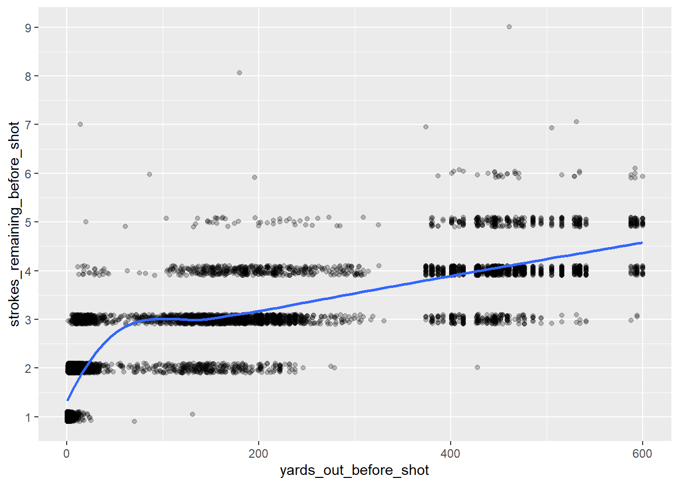

#Calculate R-Squared
cor(shots$yards_out_before_shot, 
    shots$strokes_remaining_before_shot)^2

[1] 0.682005

While there is a certainly a strong correlation between these numbers, the relationship is not quite linear. A log transformation should clean this up.

shots <- shots %>% 
  mutate(log_yards_out_before_shot = log(yards_out_before_shot+1))
  

shots %>% 
  ggplot(mapping = aes(x = log_yards_out_before_shot,
                       y = strokes_remaining_before_shot)) +
  geom_jitter(width = 0,
              height = 0.1,
              alpha = 0.1) +
  geom_smooth(method = loess,
              se = FALSE) +
  scale_y_continuous(breaks = 1:10)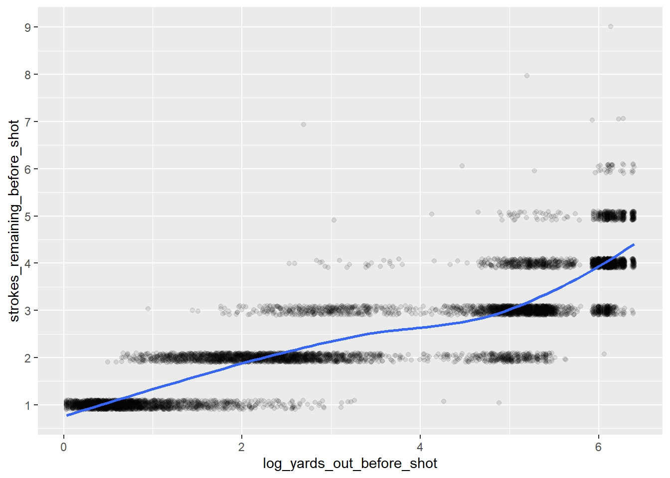

#Calculate R-Squared
cor(shots$log_yards_out_before_shot, 
    shots$strokes_remaining_before_shot)^2

[1] 0.7876248

The log transformation improves the R² value, but it can probably be improved even further with a nonlinear model. To test this, I’ll use cross-validation to evaluate out-of-sample performance. Ideally, I’d like to use some type of time-series data splitting here to avoid any possible data leakage issues², but I’ll use a simpler method in this post. I’ll split the 30 golfers into 10 groups of 3, and hold out one of these groups in the cross-validation process.

player_cv_groups <- shots %>% 
  select(player) %>% 
  unique() %>% 
  arrange(player) %>% 
  mutate(cv_group = cut_number(x = player, 
                               n = 10,
                               labels = FALSE))

shots <- shots %>% 
  inner_join(player_cv_groups,
             by = "player")

shots %>% 
  group_by(cv_group) %>% 
  summarize(golfers = n_distinct(player),
            shots = n())

# A tibble: 10 × 3
   cv_group golfers shots
      <int>   <int> <int>
 1        1       3   834
 2        2       3   840
 3        3       3   832
 4        4       3   834
 5        5       3   820
 6        6       3   835
 7        7       3   839
 8        8       3   845
 9        9       3   834
10       10       3   835

folds <- group_vfold_cv(data = shots,
                        group = cv_group)

Now, using these folds, I’ll find a performance baseline using the linear model above.

just_log_yards_recipe <- recipe(formula = strokes_remaining_before_shot ~
                                  log_yards_out_before_shot, 
                                data = shots)

lm_mod <- linear_reg(mode = "regression",
                     engine = "lm")

lm_workflow <- workflow() %>%
  add_recipe(just_log_yards_recipe) %>%
  add_model(lm_mod)

lm_rs <- fit_resamples(object = lm_workflow,
                       resamples = folds,
                       control = control_resamples(save_pred = T))

lm_rs %>%
  collect_metrics() %>%
  select(.metric,
         mean) %>%
  as.data.frame()

  .metric      mean
1    rmse 0.5569516
2     rsq 0.7900181

As expected, the mean hold-out performance is very similar to the linear model fit on all the data.

XGBoost Model

Next I’ll try a gradient boosted tree model using the XGBoost library. I love XGBoost. It trains and tunes relatively quickly, and you don’t usually need to worry about other tedious pre-processing steps like centering, scaling, and imputing. Since XGBoost is nonlinear, I wont need to use the log transformation, and can switch back to just using yards_out_before_shot.

just_yards_recipe <- recipe(formula = strokes_remaining_before_shot ~
                              yards_out_before_shot, 
                            data = shots)

xgb_mod <- boost_tree(mode = "regression",
                      engine = "xgboost")

xgb_workflow <- workflow() %>%
  add_recipe(just_yards_recipe) %>%
  add_model(xgb_mod)

xgb_rs <- fit_resamples(object = xgb_workflow,
                        resamples = folds,
                        control = control_resamples(save_pred = T))

xgb_rs %>%
  collect_metrics() %>%
  select(.metric,
         mean) %>%
  as.data.frame()

  .metric      mean
1    rmse 0.5236481
2     rsq 0.8142939

The XGBoost model improves performance without any parameter tuning, so hopefully I can get more out of it. First, I’ll look at the out-of-sample predictions,

rs_preds <- xgb_rs %>% 
  collect_predictions() %>% 
  select(row_id = .row,
         fold = id,
         pred = .pred)

preds_join <- shots %>% 
  as.data.frame() %>% 
  mutate(row_id = row_number()) %>% 
  inner_join(rs_preds,
             by = "row_id") 

preds_join %>% 
  ggplot(mapping = aes(x = yards_out_before_shot,
                       y = pred,
                       color = fold)) +
  geom_point()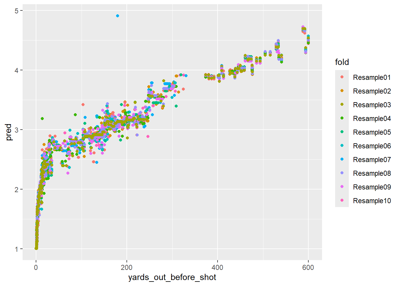

The fits look good, but the nonlinear warts are showing. This model only uses one feature, yards_out_before_shot, but the predictions vary significantly at the same distance. For example, looking at the shots around 200 yards out, the predictions vary from 2.8ish to 3.5ish. This will cause confusion when we start attributing strokes gained to specific shots.

Monotonic Constraints

Luckily, there is a fix - XGBoost has the ability to enforce monotonic constraints, meaning I can force predicted strokes remaining to increase as yards out increases. I’ll retrain my model.

xgb_mod <- boost_tree(mode = "regression") %>% 
  set_engine(engine = "xgboost",
             monotone_constraints = c(1))

xgb_workflow <- workflow() %>%
  add_recipe(just_yards_recipe) %>%
  add_model(xgb_mod)

xgb_rs <- fit_resamples(object = xgb_workflow,
                        resamples = folds,
                        control = control_resamples(save_pred = T))

xgb_rs %>%
  collect_metrics() %>%
  select(.metric,
         mean) %>%
  as.data.frame()

  .metric      mean
1    rmse 0.5201534
2     rsq 0.8168157

The model performance actually improved slightly with the constraints, which is encouraging. Now I’ll look at the out-of-sample predictions again.

rs_preds <- xgb_rs %>% 
  collect_predictions() %>% 
  select(row_id = .row,
         fold = id,
         pred = .pred)

preds_join <- shots %>% 
  as.data.frame() %>% 
  mutate(row_id = row_number()) %>% 
  inner_join(rs_preds,
             by = "row_id") 

preds_join %>% 
  ggplot(mapping = aes(x = yards_out_before_shot,
                       y = pred,
                       color = fold)) +
  geom_point()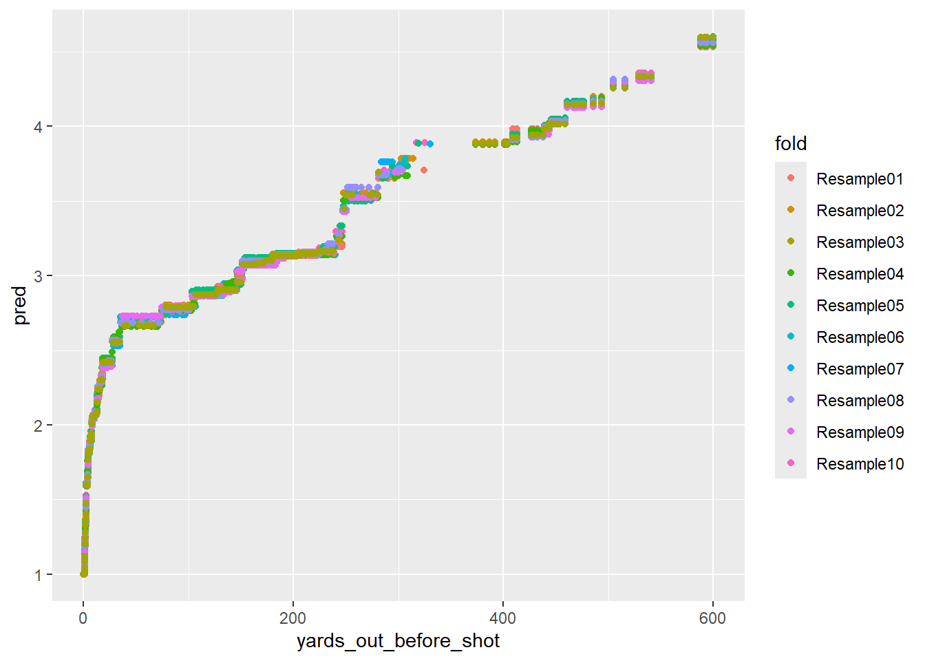

Much better! Another interesting finding is that there is a “jump” in the predictions around 260 yards. The predicted strokes remaining jump from 3.2ish to 3.5ish. This could be because it’s near the range where PGA Tour players can take more aggressive shots at the green to reduce their score. This is a good demonstration of the value of nonlinear models.

Ball Location Features

Next, I’d like to add some more features. I’ll start with the ball location (fairway, green, etc.). I cleaned up ball location data in my last post, but those were the to_location columns. Here I need the from_location columns because I am using strokes_remaining_before_shot and yards_out_before_shot.

shots %>% 
  group_by(from_location_scorer,
           from_location_laser) %>% 
  summarize(rows = n(),
            .groups = "keep") %>% 
  arrange(desc(rows)) %>% 
  as.data.frame()

   from_location_scorer            from_location_laser rows
1                 Green                        Unknown 3546
2               Tee Box                                2162
3               Fairway                   Left Fairway  550
4               Fairway                  Right Fairway  533
5         Primary Rough                     Left Rough  415
6         Primary Rough                    Right Rough  375
7    Intermediate Rough             Right Intermediate  144
8    Intermediate Rough              Left Intermediate  112
9        Fairway Bunker                        Unknown   92
10    Green Side Bunker        Right Green Side Bunker   77
11    Green Side Bunker  Right Front Green Side Bunker   66
12    Green Side Bunker   Front Left Green Side Bunker   59
13    Green Side Bunker         Left Green Side Bunker   47
14    Green Side Bunker Front Center Green Side Bunker   34
15               Fringe                   Left Fairway   28
16                Other                        Unknown   20
17        Primary Rough                        Unknown   20
18               Fringe                  Right Fairway   18
19          Native Area                     Left Rough   13
20          Native Area                        Unknown   13
21          Native Area                    Right Rough   11
22    Green Side Bunker    Left Rear Green Side Bunker    3
23                Other                     Left Rough    3
24                Green                                   2
25                Other                    Right Rough    2
26                Water                        Unknown    2
27    Green Side Bunker   Right Rear Green Side Bunker    1

shots <- shots %>% 
mutate(from_location = case_when(from_location_scorer == 'Green' 
                                 ~ 'Green',
                                 from_location_scorer == 'Tee Box' 
                                 ~ 'Tee Box',
                                 from_location_scorer %in% c('Fairway',
                                                             'Fringe') 
                                 ~ 'Fairway',
                                 from_location_scorer %in% c('Primary Rough',
                                                             'Intermediate Rough') 
                                 ~ 'Rough',
                                 from_location_scorer %in% c('Fairway Bunker',
                                                             'Green Side Bunker') 
                                 ~ 'Bunker',
                                 TRUE 
                                 ~ 'Other')) %>% 
  mutate(from_location = factor(from_location,
                                ordered = T,
                                levels = c("Green",
                                           "Fairway",
                                           "Tee Box",
                                           "Rough",
                                           "Bunker",
                                           "Other")))

shots %>% 
  filter(player == 1810,
         round == 1,
         hole %in% 1:3) %>%
  select(hole,
         shot,
         to_location,
         from_location) %>% 
  arrange(hole,
          shot) %>% 
  as.data.frame()

   hole shot to_location from_location
1     1    1       Rough       Tee Box
2     1    2       Green         Rough
3     1    3       Green         Green
4     1    4        Hole         Green
5     2    1       Green       Tee Box
6     2    2        Hole         Green
7     3    1     Fairway       Tee Box
8     3    2       Green       Fairway
9     3    3       Green         Green
10    3    4        Hole         Green

Now I’ll train a new XGBoost model with this feature. Since I’ve updated the data set, I’ll need to recreate the fold index and the recipe. I’ll use step_dummy() to convert from_location from a factor to binary terms for each location type.

folds <- group_vfold_cv(data = shots,
                        group = cv_group)

with_location_recipe <- recipe(formula = strokes_remaining_before_shot ~
                                 yards_out_before_shot +
                                 from_location,
                               data = shots) %>% 
  step_dummy(from_location)

xgb_mod <- boost_tree() %>% 
  set_mode("regression") %>% 
  set_engine("xgboost",
             monotone_constraints = c(1)) %>% 
  translate()

xgb_workflow <- workflow() %>%
  add_recipe(with_location_recipe) %>%
  add_model(xgb_mod)

xgb_rs <- fit_resamples(object = xgb_workflow,
                        resamples = folds,
                        control = control_resamples(save_pred = T))

xgb_rs %>%
  collect_metrics() %>%
  select(.metric,
         mean) %>%
  as.data.frame()

  .metric      mean
1    rmse 0.5124754
2     rsq 0.8221943

Not much of an improvement, but the model got a little better.

rs_preds <- xgb_rs %>% 
  collect_predictions() %>% 
  select(row_id = .row,
         fold = id,
         pred = .pred)

preds_join <- shots %>% 
  as.data.frame() %>% 
  mutate(row_id = row_number()) %>% 
  inner_join(rs_preds,
             by = "row_id") 

preds_join %>% 
  ggplot(mapping = aes(x = yards_out_before_shot,
                       y = pred,
                       color = from_location)) +
  geom_point() +
  scale_color_manual(values = cut_colors) + 
  labs(title = "Out-Of-Sample Predicted Strokes Remaining")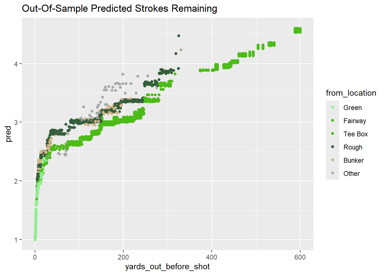

These new predictions make sense. Shots from the rough/bunker are harder and thus the predicted strokes remaining are higher. For example, at 100 yards, being in the rough (vs. fairway) increases expected strokes from 2.7ish to 3.0ish.

Adding these features increased the prediction “noise” at each distance - similar to the results of the unconstrained XGBoost model. This stems from the variation in how each sub-model handles the new features, and it goes away if I filter down to a single hold out set (Fold 1).

preds_join %>% 
  filter(fold == 'Resample01') %>% 
  ggplot(mapping = aes(x = yards_out_before_shot,
                       y = pred,
                       color = from_location)) +
  geom_point() +
  scale_color_manual(values = cut_colors) + 
  labs(title = "Out-Of-Sample Predicted Strokes Remaining",
       subtitle = "Fold 1")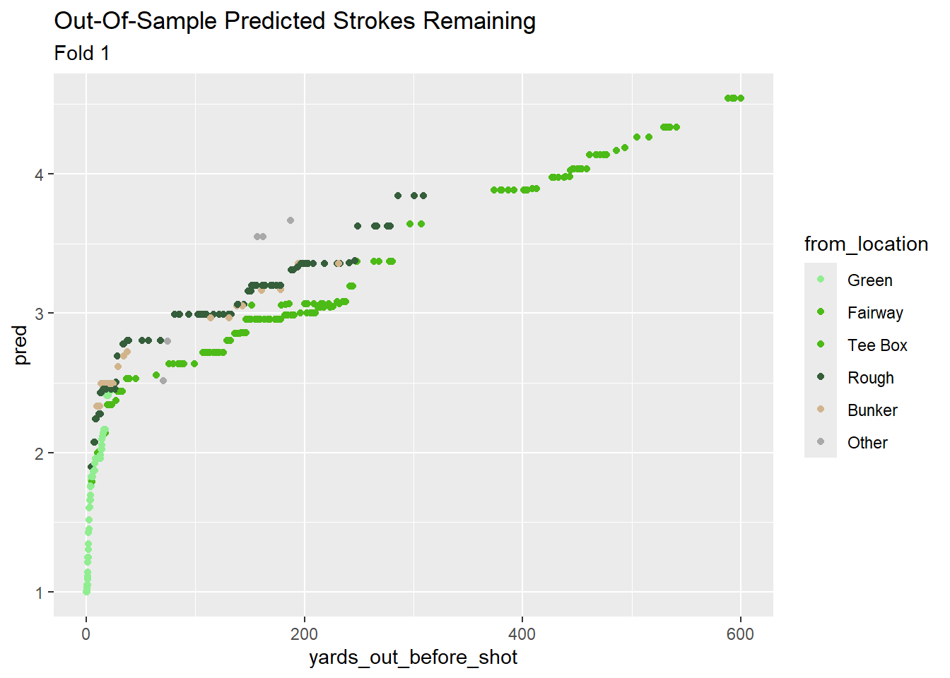

I could probably improve model performance with some parameter tuning, but I’ll stop here for now.

Footnotes

These methods have a major shortcoming in that they attribute the entire residual to a single golfer (or the teams involved). This could probably be corrected with a hierarchical/mixed model, but I’ll save that for a future post.↩︎
If I wanted to use this model to predict strokes remaining for future shot’s, I would want to make sure I’m not using future shots when training/evaluating my model.↩︎